If you have a model with multiple locations and / or periods, you may want to create limits that control not only the individual options but also sub-totals across all or some of these places and times. For example, if you have 3 locations and 3 periods in which you can buy a stream (or sell it or inventory it or transport it) there will be 9 variables to optimize. I will refer to these as L1P1, L1P2, L1P3, L2P1, L2P2, L2P3, L3P1, L3P2 and L3P3. How many constraints would you need to cover every possible sub-set? There would be 9 limits for each single possibility and 1 limit for the whole set. In between, there are the sets of 2, 3, 4, 5, 6, 7 and 8 items. The formula
 |
where n is the total set and k the size of the desired sub-set, will give us the total number of combinations with at least 1 member. In Excel you could calculate the value for each k as =FACT(n)/(FACT(k) * FACT(n-k)) – but there is also the very handy =COMBIN(n,k). |
Add them up and you will find that there are 511 possibilities Let's see how to put them in a model, starting with the 9 limits on the indvidual variables.
I can use ** as a wild-card for the period code to define three period-specific limits with a single row as long as all the data is the same, or give explicit codes to make each period different. (With table based input these would appear in TABLE 1BU.0). I set a minimum on each equal to the number of constraints defined so far as a way of counting them. 9 down, 502 to go. These will appear in the matrix as column bounds since they each involve only one variable.

In Multi-Limits (TABLE 1BU.1) the special XX code can be used for the location or period to indicate a sum over all. So the first row with its XX-XX generates the 9 member set of all options. The second row generates totals over location for each period: {L1P1, L2P1, L3P1}, {L1P2, L2P2, L3P2} and {L1P3, L2P3, L3P3}. The rows with explicit locations and XX for period are counting the totals over periods at each site: {L1P1, L1P2, L1P3}, {L2P1, L2P2, L2P3} and {L3P1, L3P2, L3P3}. 16 limits set, 495 remaining.


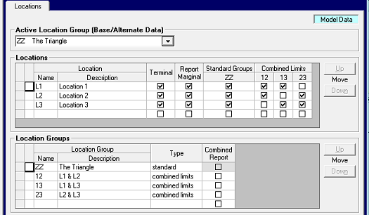
The first constraint, 12-**, makes a sub-total of purchases at L1 and L2 for each period, covering the three two-member sub-sets: {L1P1, L2P1}, {L1P2, L2P2} and {L1P3, L2P3}. With XX for the period code, the limit becomes a total of all of those together: {L1P1, L2P1, L1P2, L2P2, L1P3, L2P3}. Likewise for the other two groups, bringing our constraint total up to 28; 483 more to do.

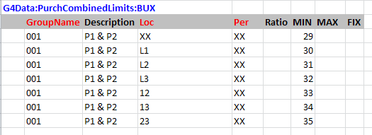
The group code is any three characters of your choice – it is not a stream, but it will save confusion if you can avoid duplicating a stream name. I’m going to use numbers for the names in this example as I expect I am going to need quite a few. It’s a good idea to define the group and members in the base case, so that they are available and, by default, consistent in all alternate cases (so no m’s in the membership grid). Groups are ignored if there is no limit on them – and limits can easily be set and changed in the alternate cases. If you are working with table input data, the group is the column for TABLE 1BU.3 and the members are the rows. As the panel will only display two rows at a time, here is the SSI sheet, showing all seven of the limits that can be set with Group 001.

Here an XX for location means that members from any location can be included. This might not be all of the active locations in the case. The same for periods. The limit defined in the first row will therefore include the 6 members: {L1P1, L1P2, L2P1, L2P2, L3P1, L3P2} but nothing for P3. The second row has an explicit location code and so will include only members at L1, for any period given: {L1P1, L1P2}. Where the location code is a group, only members with a location in that group will be taken, so 12-XX selects four members: {L1P1, L1P2, L2P1, L2P2}. There are no ** or period specific entries, since all the single period sets that could be made with these members have already been taken care of. Repeating this for the other period-pair groups adds a further 21 constraints to the model, for a total of 49; 462 remaining.
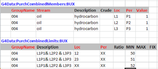
The combinations implemented so far have all been combinatorial on L X P, that is each period in the set was included for every location in the set. The remaining constraints are less symmetrical. I still need to cover things like {L1P1, L2P2} and {L1P1, L1P2, L1P3}. It is clearly going to take quite a few more groups to cover these, although somewhat less than 462, as you will see. I have, for example, given Group 004 three members and can use it for three new constraints.

The limits cover different combinations of the members, based on the location group codes. So the first row covers the set {L1P1, L2P2}, while the second is for {L2P2, L3P3} and the last has all three members {L1P1, L2P2, L3P3}. Two more groups can be made by rotating which period is selected for which location so that would be six more constraints So that’s 58 with 453 left. These remaining groups would be bigger and made by including different numbers of periods for each location. I’m not sure how many of these odder combinations would actually ever be needed in practice – perhaps for some very complicated swop deals, or transportation with delays. So at this point, I decided you probably had the idea about the whole group thing, and it was time to stop amusing myself and get on with some real work.
From Kathy's Desk 3rd May 2017.
Comments and suggestions gratefully received via the usual e-mail addresses or here.
You may also use this form to ask to be added to the distribution list to be notified via e-mail when new articles are posted.
