99) Why SLP?

One of my readers wrote to me to ask why, since we are solving non-linear problems, we use SLP instead of something like a Generalized Gradient method – as you can find in the Excel Solver. (Note that the oil industry tends to refer to planning optimization activity as LP, even though it has been decades since purely linear problems were the norm which confuses Operations Research academics and practitioners from other industries).  A lot of the reason the refinery models use SLP is history. Big oil companies were very early adopters of LP – the 1950s – and pushed the development and application of simplex algorithms very far. LP works very well for many aspects of oil /product distribution and refinery problems, so it became an industry standard.

The first non-linear problem that refinery modellers focussed on was the pooling problem. Larry Haverly, the founder of Haverly Systems, wrote a seminal paper on this: C. A. Haverly, Studies of the Behaviour of Recursion for the Pooling Problem, ACM SIGMAP Bulletin. 1978. SLP was a natural approach to try because there were simplex solvers that handled large problems and oil companies had people who knew how to use them. The DR formulation fits very neatly in to the blending variables and constraints that people were used to, so this also became a standard technique for most commercial “LP” tools during the 80s. By the turn of the century most refinery planning models were formulated as non-linear problems and pure LP models are now extremely rare.

Mr Haverly told me that people were also interested in applying other non-linear methods to solve the pooling problem– an optimizer called MINOS was available, for example – but that these were generally not very successful because refinery problems were rather large and these methods were very slow.  It just couldn’t compete against SLP. However, there have been many years of development in algorithms and computer hardware since, so it is certainly a reasonable question to ask again.  There are lots of non-linear optimization methods – and the general characteristic of them is that they make an approximation to the problem, solve it, inspect the solution and try again – just like SLP. (There is some good stuff on Wikipedia for this. For a textbook, I like Numerical Optimization by Nocedal and Wright.) So, the question then becomes, if you had access to another non-linear optimization technique, what would you gain by switching?

The Solver in Excel offers a “GRG Nonlinear” option, which is described as suitable for smooth problems. This gives us a simple environment to explore what it would be like to use a different method.   I set up a little blending problem to see how it solved, compared to the Simplex option. First, I formulated it as a completely linear problem. (I cheated a bit and used the Matrix Analyzer  to import the Blend Demo model, reduced to a single period case.)

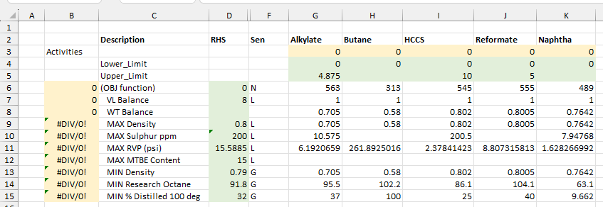
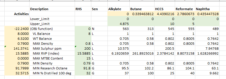
So, here we have 5 components with different costs and properties to blend into gasoline, subject to the specifications in the rows 8 through 14. The objective function in cell B7 is the SUMPRODUCT of the prices of the components and product in row 7 multiplied by the activities of the variables in row 3. It’s configured as a minimization problem with positive costs and negative revenues. The components are counted in volume.

 

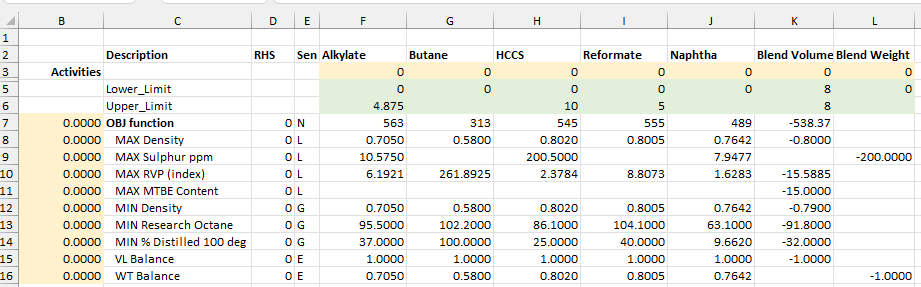
The specifications are set up as balance rows as they would be in the standard LP formulation for linear blending –

 

 

 

The positive entries for the component contributions are weighed against the specification as a negative entry on the product volume or weight (columns K and L). The weight column is needed to handle the sulphur. The volume and weight balance rows (15 and 16) are used to keep the product quantities consistent with the amount of component used. All the RHS (column D) are zero.

Configure the solver as:

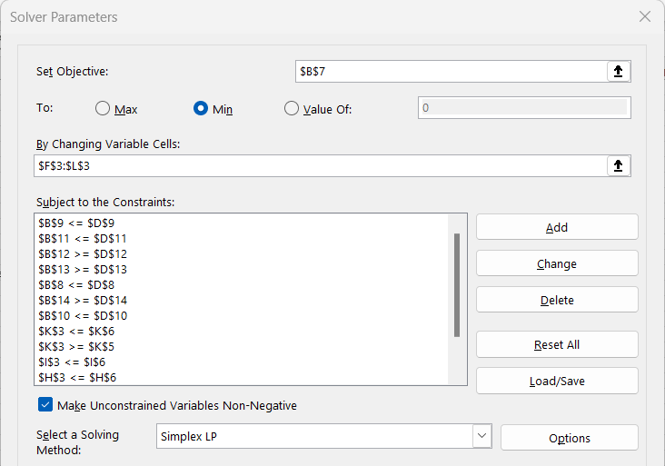
The variables are the quantities of components and blend in cells G3 to M3. As well as the specifications – the B values compared to the D values - there are also some maximum limits on the components and blend volume that are captured in the requirements that each row 3 variable be less than the amount in the corresponding column in row 6. The “Make Unconstrained Variables Non-Negative” - that is assume a lower bound of 0 - is standard for LP problems.

 

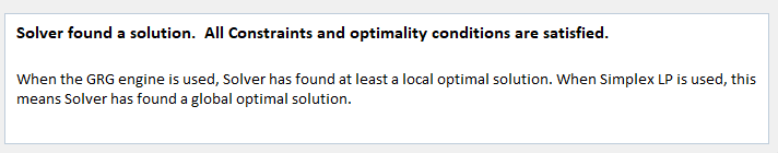
Choose Simplex LP and solve. It finds a solution very quickly.

 

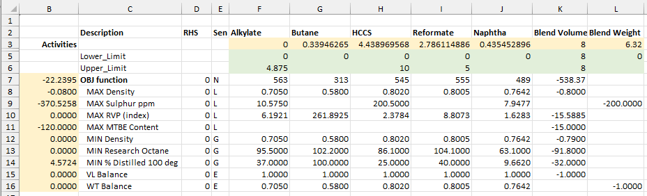
Choose the GRG Non-Linear and it finds the same solution (with trivial deviations in the component quantities). Do note the warning about local optimality that is always given, because this is an issue for almost all non-linear optimization methods (not just SLP).

 

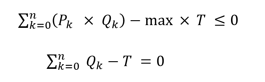
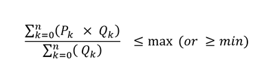
Having switched to the GRG method, we are now no longer constrained to formulating the specifications as quality balances. We can write them directly as averages with the specification as the right-hand-side. 

 

 

 

 

Once these constraints have been converted to that, the Solver will no longer let you apply the simplex algorithm.  The GRG Algorithm won’t accept the problem either, at first, because starting with all components at zero means that there are #DIV/0 errors in the specification calculations.

 

I arbitrarily set the first component to 0.01 to get rid of the error.

 

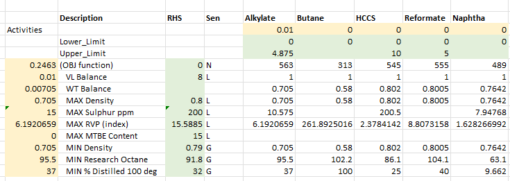
This starting point is not feasible, but the algorithm recovers to find a solution

The objective value looks a little better than what was found for the linear formulation.  Does this mean that this is the better method?   Not based on this, because the octane is actually slightly off spec.  If we relaxed the Octane spec to 91.79, the Simplex solution would also have an improved value.    This indicates that the default tolerances for feasibility/optimality are more relaxed than what the Simplex solver is using. 

 

 

Simplex	GRG

 

 

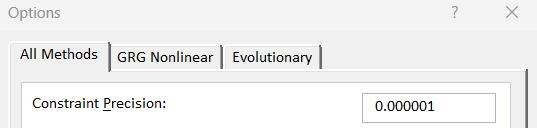
A quick check of the options confirms this.  To make a valid comparison between solvers, it is essential to ensure that they are configured to equivalent criteria.  So, I adjusted them both to 1E-06 - which is the sort of value that the large commercial solvers use - and solved again.  The octane is on spec with less rounding up and objective values are now almost the same.  

 

I noted that it was able to find a solution even when the initial assumptions were off-spec. I wondered how sensitive it would be to those assumptions, since one of the issues we have with using SLP is ending up in quite a different place depending on where it starts from.   So I played around with setting the component activities to various values.  It does make a difference to the solution - less with the tighter tolerance than with the default - but mostly trivial.  However, if you push it hard enough it will do some silly things.  For example, starting all the components are very large values often gives a solution with negative alkylate - another tolerance issue as there is a lower limit of zero.  I also found that if you started it will negative component values, it would try to set them to zero and end up stopping with the #DIV/0.   Clearly if you are going to use the solver in Excel for these kinds of problems, you need to get into the more detailed level of adjusting the tolerances and algorithm parameters.  

One would expect that a full scale commercial gradient solver would have tighter tolerances and be more robust to starting values. However, the point is well made that SLP is not unique among general non-linear optimization techniques in being sensitive to assumptions and at risk of returning poor solutions. SLP for refinery problems continue to have the advantages that the Linear element is fast and rigorous (and gives you marginal values). A significant benefit in speed or “globality” would need to be demonstrated to justify migrating to a new technique and it is by no means certain that would be the case. (Something which is also true of the idea of using AI on optimization problems) So the refinery industry continues to use SLP for their “LP” activities.